HYDROLOGY – ESTIMATION OF MISSING PRECIPITATION

There are two common methods which are used to calculate missing precipitation.

1. Arithmetic average method

This method is used if the normal annual rainfall of the missing station is within 10% of the normal annual rainfall of surrounding stations, data of at least 3 surrounding stations (index stations) are available, and the index stations are evenly spaced around the missing station and are as close as possible. The formula for computing the rainfall of a missing station is.
$P_x=1/n(P_1+P_2+P_3+⋯.+P_n)$

Where,
P₁, P₂,…, P_n: rainfall of index stations
Px: rainfall of the missing station
n: number of index stations

2. Normal ratio method

This method is used when the normal annual rainfall of the index stations differs by more than 10% from that of the missing station. The rainfall of the surrounding index stations is weighted by the ratio of normal annual rainfall by using the following equation:

$P_x=1/n (N_x/N_1 P_1+N_x/N_2 P_2+N_x/N_3 P_3+⋯.+N_x/N_2 P_n )$
$=N_x/n (P_1/N_1 +P_2/N_2 +P_3/N_3 +⋯.+P_n/N_2 )$

Where,
P₁, P₂,…, P_n: rainfall of index stations
P_x: rainfall of the missing station
n: number of index stations
N_x: normal annual rainfall of the missing station
N₁, N₂,…., N_n: normal yearly rainfall of index stations

Double mass curve analysis for correction for data inconsistencies

The plot of the accumulated annual rainfall of a particular station versus the accumulated annual values of the mean rainfall of surrounding stations is called a double mass curve. This technique is used to check the consistency of rainfall data and to correct erroneous rainfall data. This technique is based on the principle that a group of sample data drawn from its population will be the same. The reasons for inconsistency are:
– Shifting of gauge
 – Change in site conditions due to calamities, e.g., fires, landslides
 – Change in observational procedure
 – Observation error
If the double mass curve is a straight line, the rainfall of the particular station is said to be consistent. If there is a break in the slope of the plot, then the rainfall of that particular station is inconsistent. The starting year of the change of regime of rainfall is marked by the starting point of the break in slope. Correction has to
be applied beyond the period of change of regime.


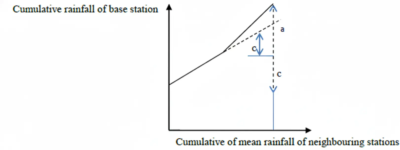
Fig.: Double Mass Curve

Steps in double mass construction:
 a. Select a group of 5 to 10 neighbouring stations
 b. Arrange data in chronological order with the latest data in the beginning.
 c. Compute the cumulative rainfall of the base station (the station whose consistency is to be checked).
 d. Compute the cumulative mean rainfall of neighbouring stations.
 e. Plot the cumulative rainfall of the base station versus the cumulative mean rainfall of neighbouring stations, and join the points by a straight line.
 f. Check if there is a break in a straight line.

The formula for the correction for rainfall after a line break is given by:

$P_cx=P_x (M_c/M_a)$

Where,
P_cx = Corrected precipitation for station x
P_x: Original precipitation of station x
M_c: Slope of original line
M_a: Slope of the line after the change of regime
If c and a are the vertical intercepts of the original line and the line after the change

And,
$P_cx=P_x (c/a)$
A change in slope is normally taken as significant only where it persists for more than five years. A correction should be applied for a change in slope exceeding 10% of the original line.

Presentation of rainfall data

a. Rainfall depth
 – Rainfall intensity: rainfall depth/time interval.
b. Point rainfall
 – Rainfall data of a station for a certain duration.
 – Duration: Hourly, Daily, Weekly, Monthly, Seasonal, Annual.
 – Plot: Rainfall versus time in a bar diagram.
c. Moving average
 – Average of consecutive intervals.
 – Interval: 3-5 years.
 – Purpose: to isolate the trend in rainfall data and to smooth out the high-frequency fluctuations.
d. Mass curve
 – Plot of accumulated rainfall versus time.
 – Useful to identify intensity, duration, magnitude, and starting and ending time of rainfall.
 – Magnitude = cumulative rainfall at t – cumulative rainfall at t-1.
- Intensity = slope of the curve.

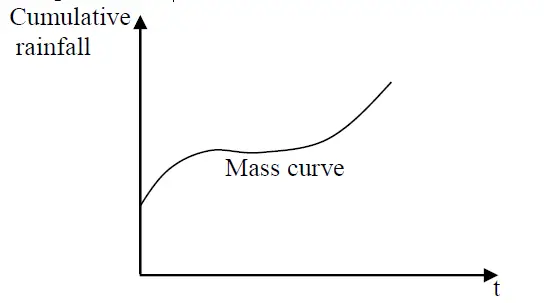
Fig.: Mass curve of rainfall
e. Hyetograph
 – Plot of rainfall intensity or rainfall depth versus time interval in the form of a bar graph.
 – In each bar, the time interval between two points is shown on the X-axis, and the corresponding rainfall represents the Y-axis.
 – From the mass curve, rainfall of a certain interval dt can be computed, and rainfall intensity can be obtained.
 – The graph represents the characteristic.

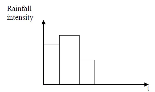
Fig.: Hyetograph

Method of computing average rainfall

1. Arithmetic mean method

This is the simplest method for computing mean rainfall. This method is satisfactory if the gauges are uniformly distributed and the individual gauge catches do not vary greatly about the mean. The formula for computing the mean rainfall is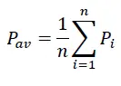
$P_av=1/n ∑_(i=1)^nP_i$

Where,
P_av = average rainfall
n = number of stations
P_i = precipitation of station i

This method gives equal weights to each gauge. It gives only a rough estimate. It does not take into account the topography and other influences. For this method, only the gauges inside the basin are considered.

2. Thiessen polygon method

In this method, weightage is given to all the gauges on the basis of their area coverage. The Thiessen method assumes that rainfall at any point within the polygon is the same as that of the nearest gauge. For this method, all the gauges in and around the basin are considered.

Method of constructing a Thiessen polygon
 – Draw a map of the basin and locate the rainfall stations.
 – Connect the adjacent rainfall stations by straight lines, forming triangles.
 – Draw perpendicular bisectors to each of the sides of the triangle lines. The perpendicular bisectors form the boundary of polygons. Wherever the basin boundary cuts the bisectors, it is taken as the outer limit of the polygon.
 – Measure the area of each polygon which surrounds a station. Area can be computed by using formulae for a regular geometric figure. For an irregular figure, the area is determined by using a planimeter or by tracing on a graph and counting squares.

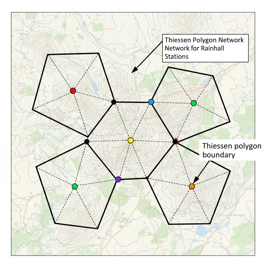
Fig.: Method of constructing a Thiessen polygon
The formula to compute mean rainfall is


Where,
P_av = average rainfall
P_i = Rainfall of station i
A_i = Area of polygon which encloses station i
A Total basin area
A_i/A: Weight for station i = w_i
$P_av=∑_(i=1)^n〖W_i 〖WP〗_i 〗$

Advantages
 – Use of data from the nearby stations located outside the basin.
 – Consideration of the spacing of stations.
 – Easy to perform computation through computer software.

Limitations
 – It does not consider orographic and topographic effects.
 – The method assumes a linear variation of precipitation between stations.

3. Isohyetal method

An isohyet is a line joining points of equal rainfall. For this method, rainfall stations lying within the basin, as well as nearby stations around the basin, are considered.

Method of constructing isohyetas
 – Draw a map of the basin and locate the rainfall stations.
 – Mark the depth of rainfall at each station.
 – Draw isohyetas by interpolating between adjacent gauges and considering orographic, storm characteristics and other factors.
 – Measure the area between successive isohyets.

The mean rainfall is computed by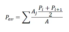


Where,
P_av = average rainfall
P_i, P_i+1: rainfall of isohyets i and i+1
A_j = Area enclosed by isohyets i and i+1
A = Total basin area
Note: if the isohyets go out of the boundary, then the catchment boundary is used as the bounding line.


Fig.: Example of Isohyetal Method
Advantages
 – Data from nearby stations located outside the basin can also be used.
 – Spacing of stations, as well as the magnitude of precipitation, is considered in the method.
 – The method is more accurate due to the consideration of topography and other influences.

Limitations
 – The method requires a dense gauge network.
 – Isohyets need to be drawn for each storm.

Intensity-duration-frequency (IDF) curve

An intensity duration frequency (IDF) curve is a three-parameter curve in which duration is taken on the x-axis, intensity on y-axis and the return period or frequency as the third parameter. The IDF curve is a very important tool for the determination of runoff, which is required for design. The curve can be used to determine the rainfall intensity for other durations with a given intensity of a particular duration.

IDF Curves by frequency analysis
When observed rainfall data of different durations are available, IDF curves can be developed using frequency analysis.

Method
For each duration selected, e.g. 15 min, 30 min, 1hr, etc., extract annual maximum rainfall data from
historical record.
For each duration, perform frequency analysis, i.e. find rainfall values of different return periods such as 2,
5, 10, 25, 50, 100 yr. (Return period is the average interval of time within which an event of given
magnitude will be equalled or exceeded.)

The steps involved in the simple plotting position method, which can be used for precipitation data, are given below.
 – Prepare data of maximum intensity for different durations for different years.
 – Arrange data in descending order.
 – Assign rank of data. Assign 1 for the highest data, 2 for second second-highestthe data and so on.
 – Calculate the return period of each data. According to California formula, return period (T) = n/m, where n = number of data, m = rank.
 – Plot rainfall versus return period and extrapolate to get rainfall of higher return periods.


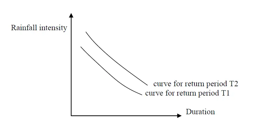
Fig.: IDF Curve

Intensity of rainfall decreases with the increase in duration of storms and increases with the increase in the frequency of storms. IDF curves can be expressed as equations in the exponential form given by


Where,
i= intensity
T = return period or frequency
D = Duration
K, x, a, n = Constants

Depth Area Duration (DAD) Curve

A Depth-Area-Duration (DAD) curve is a graphical representation of the depth of precipitation and area of its coverage, with duration of occurrence of the storm as the third parameter. Storms of smaller duration have smaller depth, and the depth decreases with an increase in area.
The purpose of the DAD curve is to determine the maximum amount of precipitation that has occurred over various sizes of drainage area during the passage of storm periods of say 6 hours, 12 hours, 24hr or other durations. Such information is essential for the design of hydraulic structures such as reservoirs, dams, culverts etc.

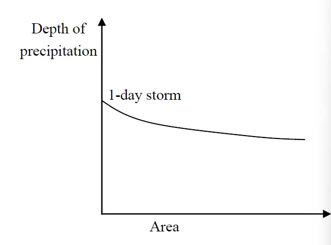
Fig.: DAD Curve
The incremental isohyetal method is generally used to construct the DAD curve. The procedure of this method is as follows.
– Identify all the major storms.
– Note down the duration for all storms, such as 1 day.
– Prepare isohyetal pattern for all 1-day storms on the map.
– Take one 1-day storm and calculate the area bounded within the highest isohyets by planimetering. Next, compute the area bounded between the largest and second largest isohyets by planimetering. Repeat the procedure for the remaining isohyets. Compute average isohyetal depth (Pmi). This procedure is repeated for all other 1-day storms in the area. The average depth of precipitation is computed as follows.


where d_n = average depth of precipitation covering up to nth isohyets, P_mi = average isohyetal depth for i^th
isohyets, A_i = Area enclosed between i^th and (i+1)^th isoheytas.
Plot a graph between cumulative area as abscissa and maximum average depth of precipitation as ordinate covering the depth area data of all 1-day storms.

The same procedure as explained above is applied for other durations.

The DAD curve can be expressed by an empirical equation as:

$P=P_0 e^(〖-KA〗^n )$
Where,
P depth of rainfall over an area of A, P₀ = rainfall at the center of the rainfall, k and n = constants

Snowfall and its measurement

The atmospheric requirements for snowfall
 – Presence of water vapour
 – Presence of ice nuclei
 – Ambient temperature below 0⁰C

Ice nuclei: particles that cause ice crystals to form through either direct freezing of cloud droplets or freezing of water deposited on the particle surface as vapour. E.g., dust particles, combustion products, organic matter
Once ice crystals form, they may splinter and create a large number of nuclei to aid the precipitation process. Continued growth of an ice crystal leads to the formation of a Snow crystal.
Snow pellets.
Snowflake: an aggregation of snow crystals, may grow in size during its falling

Snowfall or rainfall from snowflakes depends upon the extent and temperature of the layers of air through which it
falls.

Variables
 – Depth of snow
 – Snow water equivalent
Snow water equivalent is the amount of water that would be obtained if the snow were melted.
 – Density of snow
It is the percentage of snow volume that would be occupied by its water equivalent.
Density = volume of melt water from a snow sample/initial volume of sample

Snow water equivalent = Depth of snow x Density of snow
Density: in terms of a fraction
If the density of water and the density of snow are given,
Snow water equivalent = Depth of snow x (Density of snow/Density of water)
Where,
Density of new snow: 0.01-0.15,
damp new snow: 0.1-0.2,
settled snow: 0.2-0.3

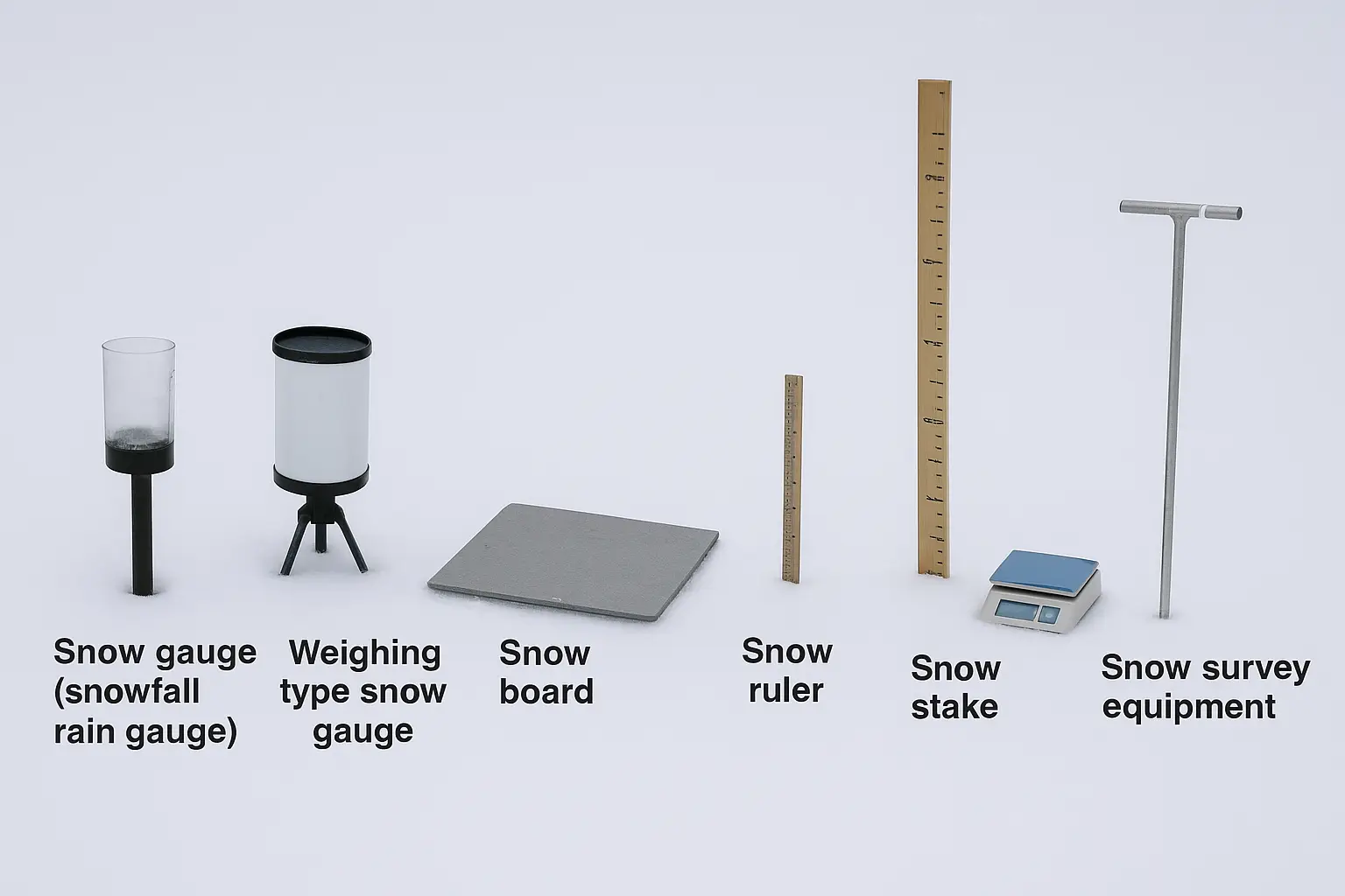
Measurement of snow
1. Point snowfall water equivalent: Snow is collected in a rain gauge (non-recording, weighing type), which is melted, and the equivalent amount of water is measured.
2. Point snowfall depth: Ruler, snowboard
Snow accumulated on the snowboard is measured by a scale or ruler
3. Snow depth for the area having large accumulation: permanent snow stakes (calibrated wooden posts fixed on the ground)
4. Areal snow cover depth and density: Snow survey
Snow survey means surveying sections of snow cover to determine depth and density.

Depth determination: by preinstalled gauges
Density determination: boring a hole through the snowpack or into the pack and measuring the amount of liquid water obtained from the sample.

Installation of Snow Guage and convert into snow water equivalent (SWE)

– Place a snow gauge in an open area.
– away from: Buildings, Trees, Slops, etc.
– Height of gauge mouth: About 30-50 cm above ground
– Ensure the gauge is vertical and stable: To avoid wind turbulence and obstruction errors.
– Add anti-freeze and a thin oil layer inside the gauge to prevent freezing, snowfall, gauge and evaporation.
– Allow collect to collet directly in the actual millimetres reading during the observation period.
– After snow fall, melt the collected snow carefully and measure the melted water using a measuring cylinder or weiging mechanism.
– record the reading in SWE as snow water equivalent (SWE), which represents the actural precipitation.

SWE= Depth of snow x Density of Snow
Example : Snow depth = 300mm and Density of snow is =0.2
than,
SWE =300 x 0.2 =60 mm